Maybe it was to test the limits of my current abilities, prove to myself that I haven’t forgotten the essence of engines, and prepare for spring recruitment; maybe it was inspired by Animal Well, Games104, etc.; or maybe it was because recently I dissected Godot and Jolt’s design and it didn’t seem that difficult. Anyway, I started writing my own small engine, and at the turn of the new year, I achieved some initial results, hence this series.
Most readers here should be insiders, so I’ll briefly introduce the features: tree-structured organization of objects, components adding functionality, scene serialization for saving and loading. Rendering uses OpenGL + GPU Instancing, simulation uses a thread pool with work stealing. Let me also explain the name and icon. The name is the same as the Pokémon Ditto, because I initially planned to focus on physics simulation, as I personally value interactive experiences in games, which technically translates to simulation and animation in graphics. The icon image is mainly inspired by Duoling from Rock Kingdom, a pet released around the time I quit that browser game. I really liked its background setting as “the legendary collector of souls, shaping its own body by absorbing the souls of other pets.” When designing the engine’s functional architecture, I often drew inspiration from mature engines.
Preparation
First, before writing, you should have a basic understanding of engine architecture and your own capabilities. According to Games104, an engine should contain 5 layers:
Function Layer: Provides basic services on the engine surface. Rendering, Game Tick, values, etc.
Tool Layer: Provides interactive editing content for developers.
Core Layer: Provides underlying support. For example, memory management and vector calculations commonly used in 3D engines.
Resource Layer: Manages creation assets.
Platform Layer: Provides cross-platform support.
The platform layer is obviously beyond the scope of a small engine like mine. Handling various images, videos, audio, models in the resource layer would be very time-consuming and labor-intensive; maybe using libraries could help, but let’s set that aside for now. The other three layers are essential for the engine to run. The current project code is also organized according to this architecture.
With the basic architecture in place, the first step is naturally to handle rendering. No matter what you do, it only gets seen when rendered. Compared to the scene, I worked on the UI interface first, because the UI is on top of the scene and is seen first, and having an Editor interface makes the whole thing look more like an engine.
Preparation
Implementing various text, buttons, input boxes by myself would be too time-consuming and labor-intensive, and the aesthetics would be questionable. So I went with IMGUI, which has multiple underlying options like OpenGL, DirectX, Vulkan. All controls are manually specified and implemented, and performance is excellent. There is also a dedicated website demo showing what it can achieve. The basic usage is as follows, somewhat similar to Unity Editor writing.
Generally speaking, an engine will have interfaces like Tool, Scene, Game, Hierarchy, File, Inspector, etc. I don’t want to implement the resource layer, so I’ll ban File; I don’t want to implement multiple views, so I’ll merge Scene and Game. Roughly here I only need to implement the Tool toolbar, Hierarchy, Scene view, and Inspector.
Starting from the top toolbar, since various extensions are not considered, the toolbar only has functions for saving/loading scenes and showing/hiding interfaces.
if (ImGui::BeginDragDropTarget()) { if (const ImGuiPayload* payload = ImGui::AcceptDragDropPayload("GAMEOBJECT")) { GameObject* droppedObj = *(GameObject**)payload->Data; if (droppedObj) { if (droppedObj->parent) droppedObj->RemoveFromParent(); else { auto& rootList = engine->scene->gameObjects; auto it = std::find(rootList.begin(), rootList.end(), droppedObj); if (it != rootList.end()) rootList.erase(it); } engine->scene->gameObjects.push_back(droppedObj); droppedObj->parent = nullptr; } } ImGui::EndDragDropTarget(); }
for (GameObject* obj : engine->scene->gameObjects) DrawGameObjectNode(obj);
ImGui::End(); }
Next is the Scene view. There’s no special logic, just recording FPS and PPF (physics time per frame), since the engine focuses on physics and involves multithreading, requiring fine-grained comparison.
if (engine->state == Engine::State::Play) ImGui::BeginDisabled(); selectedObject->OnInspectorGUI(); if (engine->state == Engine::State::Play) ImGui::EndDisabled();
ImGui::End(); }
Written behind
After that, the prototypes of various interfaces come out. Here you could use IMGUI’s main branch or the docker branch; with docker you could also implement window docking, etc. But I’m lazy, so for now it’s like this.
Simulation
Written before
As mentioned earlier, we need to handle the behavior during Play, so let’s start directly. Currently, only rigid bodies are supported, because soft bodies would disrupt the mesh structure, which would break the previously written GPU Instancing (GPU Instancing: Yeah, what would I eat?). So for now, the main work of physics is collision handling. Broad phase uses AABB, narrow phase ideally would use SAT for these geometric bodies, but for extensibility I’ll go with GJK-EPA.
Preparation
Here’s a brief introduction to the aforementioned collision detection algorithms. For convenience, we’ll use 2D convex polygon examples and only cover the algorithm ideas.
Separating Axis Theorem (SAT)
The algorithm idea is simple: find an axis that separates the two objects; if none found, they collide. Using the edges of the objects as axes is the fastest. In 3D, the complexity is O(n+m) where n and m are the number of edges.
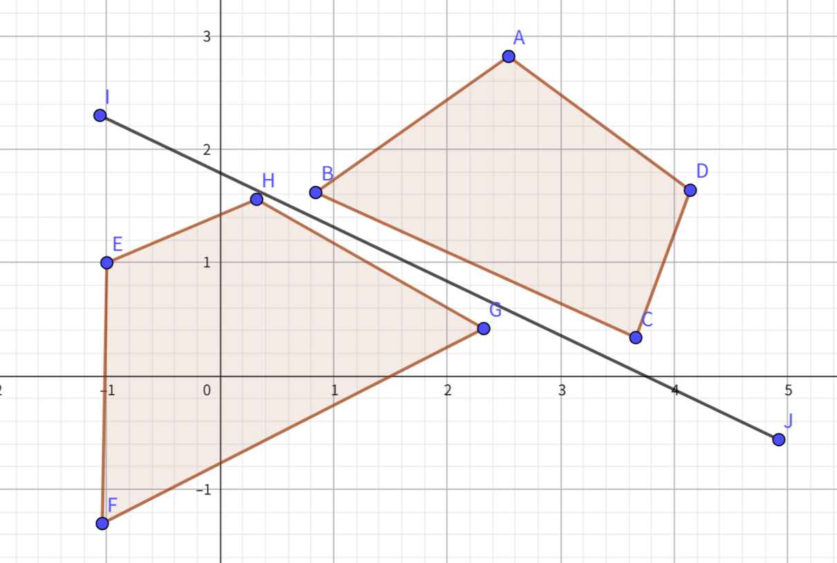
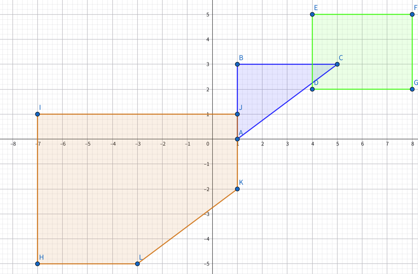
GJK-EPA
GJK involves simplices and Minkowski difference. For collision detection between the blue and green regions, we get the orange region. The orange region contains the origin, so a collision occurs. The shape of the orange region comes from the shapes of the two regions (imagine the blue region as an empty frame, the green region as a constraint – constrain a vertex of the blue region to an edge of the green region, and translate the blue region along the green region’s edges to get the red region shape), and its position comes from the relative positions of the two objects (the difference between C and D is (1,1), so point J is (1,1)). In 3D, the complexity is near constant, reaching O(n+m) only in extreme cases.
EPA is similar to GJK but instead of finding the origin, it finds the edge closest to the origin to determine penetration depth. In 3D, the complexity is O(k(n+m+f)).
Physics Stepping
Main Flow
The main flow is roughly as follows. Since we’re dealing with rigid bodies, we use the impulse approach, with position correction as an auxiliary measure to prevent continuous penetration.
voidPhysics::UpdatePhysics(float dt) { t += dt; if (t < deltaTime) return; int steps = glm::min(3.0f, t / deltaTime); t = fmod(t, deltaTime);
for (int step = 0; step < steps; ++step) { // 1. Clear previous frame's collision data collisionData.clear(); colliderPairs.clear(); // 2. Integrate forces (update velocity and angular velocity) IntegrateForce(deltaTime); // 3. Update BVH tree if (bvhTree) bvhTree->UpdateBVHTree(); // 4. Broad phase collision detection HandleBroadCollisions(); // 5. Narrow phase collision detection HandleNarrowCollisions(); // 6. Multiple iterations of sequential impulse solving for (int iter = 0; iter < iterations; ++iter) SolveCollisions(iter); // 7. Apply position correction ApplyPositionCorrections(); } // Currently physics runs at 60 FPS, rendering does not. So after each physics update, update the model matrices. for (auto collider : colliders) collider->transform->UpdateTransform(); }
Updating the BVH Tree
Here’s a brief look at the BVH tree update process. For broad-phase AABB detection, I constructed an AABB BVH tree based on SAH. Each physics frame, it updates and samples for reconstruction to maintain a relatively optimal structure.
With the BVH tree, each time we get an AABB, we can query the tree directly. But to avoid writing duplicate collision pairs, we use a flag to only include the current and its preceding AABBs.
if (!alreadyExists) if (other->rigidbody->type == RigidbodyComponent::Dynamic || other->rigidbody->type == RigidbodyComponent::Static) colliderPairs.push_back({ collider, other }); } } } }
Narrow Phase Detection
For narrow phase, we use the previously mentioned GJK-EPA. However, compared to 2D, 3D is significantly more complex. For example, when constructing the simplex, we need to handle different dimensional cases separately:
2 points (line segment): Determine the origin’s position relative to the line segment, update direction or degenerate to a single point.
3 points (triangle): Determine the origin’s position relative to each edge of the triangle, update simplex and direction.
4 points (tetrahedron): Check if the origin is inside the tetrahedron (i.e., relative to each face’s normal direction). If the origin is inside, return true; otherwise, discard the farthest face and update direction.
CollisionInfo GJK_CheckCollision(Collider* colliderA, Collider* colliderB) { CollisionInfo result; glm::vec3 direction = glm::vec3(1, 0, 0); // Initial direction
std::vector<SupportPoint> simplex; simplex.push_back(GetMinkowskiSupport(colliderA, colliderB, direction)); direction = -simplex[0].point;
for (int i = 0; i < 50; ++i) // Limit iterations to prevent deadlock { SupportPoint next = GetMinkowskiSupport(colliderA, colliderB, direction); if (glm::dot(next.point, direction) < 0) return result; // Didn't pass origin, no collision
After obtaining collision information (collision points and depth), we need to use impulses to push back. Here are the steps in more detail:
Sequential Solving and Iteration: Each frame, collisions are processed in descending order of penetration depth, and multiple iterations (e.g., 4) are used to gradually converge and reduce error accumulation.
Normal Impulse: Calculate the normal impulse based on relative velocity, restitution coefficient, and penetration depth, used to separate objects and compensate for penetration.
Tangential Friction: Calculate static and dynamic friction separately based on relative tangential velocity, limiting the tangential impulse within the friction cone to simulate surface resistance.
Rigid Body Motion Update: Impulses change both linear and angular velocities, achieving realistic rotational responses through world-space inertia tensor conversion.
The final step of pushing objects out along the penetration direction is not strictly necessary; it’s just to correct the persistent penetration caused by the impulse method. When doing physics, you could use only impulses or the PBD method, but since the impulse method is more physical, the engine primarily uses the impulse method.
voidPhysics::ApplyPositionCorrections() { for (auto& data : collisionData) { if (data.info.depth > 1e-3) { Collider* a = data.colliderA; Collider* b = data.colliderB; const CollisionInfo& info = data.info;
At this point, the engine also shows some behavior when Play is clicked, which is commendable. But as a game/physics engine, this is far from enough; at the very least, we need to try multithreading. Currently, with 2000 collision pairs in the release version, the physics frame time is 330 microseconds, and FPS drops to 400+, leaving room for subsequent comparison.
Parallelism
Written before
We have already implemented the basic physics simulation process, but its performance when dealing with a large number of collision pairs is still not satisfactory. Therefore, the next step is to try parallelization. The first step is, of course, to write a thread pool to manage threads and tasks, and then use graph coloring to avoid locking when applying impulses and position corrections.
Thread Pool
Since we’re going with a thread pool, we might as well go all the way and implement work stealing to balance the load. Here’s the general structure of the thread pool.
1 2 3 4 5 6 7 8 9 10 11 12 13 14 15
structThreadPool { structWorker { std::deque<std::function<void()>> tasks; // Task queue (deque for stealing) std::mutex mutex; // Mutex protecting the queue };
std::vector<std::unique_ptr<Worker>> workers; // Local data for all worker threads std::vector<std::thread> threads; // Worker threads std::atomic<bool> stop; // Stop flag std::atomic<size_t> next_thread_index; // Index for round-robin task assignment std::mutex cv_mutex; // Mutex for condition variable std::condition_variable cv; // Global condition variable to notify new tasks };
Chunked Synchronization
Evenly divide the range into chunks, then create tasks and submit them to the thread pool.
for (size_t t = 0; t < numThreads; ++t) { size_t blockStart = start + t * chunkSize; size_t blockEnd = std::min(blockStart + chunkSize, end); if (blockStart >= blockEnd) break;
remaining++; Enqueue([this, blockStart, blockEnd, &func, &remaining, &local_cv, &local_mutex]() { for (size_t i = blockStart; i < blockEnd; ++i) { func(i); } std::unique_lock<std::mutex> lock(local_mutex); if (--remaining == 0) { local_cv.notify_one(); } }); }
// Wait for all chunks to complete std::unique_lock<std::mutex> lock(local_mutex); local_cv.wait(lock, [&remaining] { return remaining == 0; }); }
Task Submission
When a task is added, the thread pool first performs round-robin selection and then pushes it to the back.
1
2
3
4
5
6
7
8
9
10
voidThreadPool::Enqueue(std::function<void()> task) { // Round-robin select a target thread's local queue size_t target = next_thread_index.fetch_add(1, std::memory_order_relaxed) % workers.size(); { std::unique_lock lock(workers[target]->mutex); workers[target]->tasks.push_back(std::move(task)); } cv.notify_one(); // Wake up one waiting thread }
Worker Loop
In the main loop, it preferentially takes tasks from the head of its own local queue. If its local queue is empty, it attempts to steal tasks from the tail of other threads’ queues, then executes the task or waits.
Afterwards, all steps can be rewritten using the thread pool’s chunked synchronization. However, note that during broad and narrow phase detection, the results are written to arrays. If we go parallel, merging can be done via local processing.
threadPool.parallel_for(0, numBlocks, [&](size_t blockIdx) { size_t start = blockIdx * chunkSize; size_t end = std::min(start + chunkSize, numPairs); auto& local = localData[blockIdx]; for (size_t i = start; i < end; ++i) { auto& pair = colliderPairs[i]; CollisionInfo info = GJK_CheckCollision(pair.first, pair.second); if (info.flag && info.depth > 1e-3f) { local.emplace_back(pair.first, pair.second, info); } } });
for (auto& local : localData) { collisionData.insert(collisionData.end(), local.begin(), local.end()); } }
Graph Coloring Grouping
And for lock-free impulse processing and position correction, we use graph coloring grouping. Roughly treat collision pairs as edges in a graph, and rigid bodies as vertices. Each edge needs to be assigned a color (group number) such that adjacent edges do not have the same color. The engine uses an approximate greedy algorithm to quickly generate parallelizable groups. This ensures that collision pairs within each group do not share any rigid bodies, so they can be safely solved in parallel within the group.
With this approach, in the release version with 2000 collision pairs, the physics frame time is 90 microseconds, FPS 1500+, compared to the serial version’s 330 microseconds and FPS 400+, which is a significant improvement. Of course, I have to complain that multithreading is really hard to get right. Initially, I didn’t want to write it myself, so I tried OpenMP, TaskFlow, and PPL sequentially, but their performance was comparable to serial. In the end, I had to implement multithreading myself. And after the current version, I also tried C20 barriers, hoping for further improvement, but the performance was again comparable to serial. Tired, so let’s leave it at that for now.

 wechat
 alipay