
Analysis of Godot Physics Source Code
Written before
Reading engine source code is fundamental for engine development roles, and those who know me are aware that I focus on physics simulation. During an internship at a project team, I had modified Unity’s source code, but back at school, I can only access open-source engines. UE’s Chaos is somewhat heavy: during initialization, the Scene sequentially creates Scene, Solver, Evolution, and Objects sequentially register events, create states, and initialize bodies; during simulation, AOS data from the game thread is pushed to the SOA physics thread, undergoes a series of complex calculations (considering my focus on mobile performance), and then dirty modified data is pulled back. In contrast, Godot’s source code is lightweight and well-structured, making it suitable for dissecting the 3D physics portion.
Reviewing the latest Godot 4.5 documentation is actually quite interesting. For example, Godot’s memory management: small objects use heap allocation with reserved free memory, while large objects use a dynamic memory pool (recorded using PooledList for lists and freelists). This differs significantly from the OS’s paging choices, highlighting the difference between specialization and generality? Also, Godot’s 2021 article explaining why it doesn’t use an ECS architecture and its choice of abstraction levels (offering a new perspective, though I personally don’t entirely agree, but since it’s open source, one can build their own framework if needed). Furthermore, Godot’s mobile rendering pipeline cannot read adjacent pixels (Seriously? This disables fragment derivatives, and compute shaders are largely unsupported. Even phones in India and Southeast Asia aren’t this fragile, are they?).
Architecture Overview
The entire 3D physics portion of Godot resides in modules/godot_physics_3d, making it exceptionally convenient to locate.
- Physics Server (
godot_physics_server_3d) creates and manages spaces, shapes, areas, and collision objects. - Physics Space (
godot_space_3d) contains all objects in the physics world and is responsible for physics simulation. - Physics Stepper (
godot_step_3d) is used by the space to step through the physics simulation. - Collision Detection (
godot_broad_phase_3d) quickly identifies potential colliding object pairs. - Collision Solver (
godot_collision_solver_3d) handles specific collision detection between shapes. - Shapes (
godot_shape_3d) define various geometric shapes used for collision detection. - Collision Objects (
godot_collision_object_3d) are the base classes for Areas, RigidBodies, and SoftBodies, all of which can have shapes. - Areas (
godot_area_3d) detect object entry and exit and can modify properties like gravity. - Rigid Bodies (
godot_body_3d) are hard physical objects affected by forces and collisions. - Soft Bodies (
godot_soft_body_3d) are deformable objects simulated using a particle system. - Constraints and Joints (
godot_constraint_3dandgodot_joint_3d) restrict motion between objects.
The simulation flow is roughly as follows:
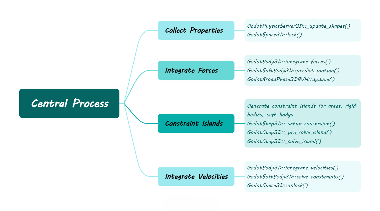
Parameter Preparation
First, let’s start with preparation. Although it involves handling various property settings, the main processing lies in updating the object’s mass properties. Taking the most complex RigidBody as an example, it first calculates the total area (summing the area of each shape), then calculates the center of mass (distributing mass proportionally by area), and finally calculates the inertia tensor (parallel axis theorem).
1 | void GodotBody3D::update_mass_properties() { |
Let’s briefly supplement the calculation of the inertia tensor:$I_{total} = \displaystyle\sum_{i=1}^{n}{(R I_{local}R^T + w(r \cdot r \cdot I_{identity} - r \otimes r))} $。Bounded by the plus sign, the left side is the current shape’s moment of inertia, and the right side is the weighted composition. This might be abstract, so let’s illustrate with the inertia tensor of a point cloud.
Assume we have a spinning top composed of n points, where the coordinates of point i are pi, the mass of point i is mi, and we wish to calculate its initial rotational inertia. Then the formula is:$I_{ref}=\displaystyle\sum_{i=1}^{n}(m_i(r_i\cdot r_i\cdot I_{identity}− r_i\otimes r_i))$,, where the offset vector $r_i=p_i-p_{center}$. This is the right part of the formula used by the engine, where the dot product describes mass distribution, and the outer product describes inertia contribution. Then the top starts spinning with rotation matrix $R$, giving $ I=RI_{ref}R^T $. This is the left part of the formula. Combining them yields the scheme used by the engine (here, the engine’s method accounts for the positional offset of the shape within the overall inertia tensor, which I personally find unnecessary).
Integrating Forces
After updating the physical properties, the next steps are integrating external forces for rigid bodies, shape prediction for soft bodies, and BVH collision detection.
Integrating Forces for Rigid Bodies
First is integrating forces for rigid bodies. Skipping the code that iterates through areas to determine damping modes, we go directly to the core part. For kinematic objects, they are externally driven, and their linear and angular velocities are updated based on position and rotation changes. For rigid bodies, they first calculate the net force and net torque, then apply damping to update velocity.
1 | void GodotBody3D::integrate_forces(real_t p_step) { |
Shape Prediction for Soft Bodies
Next is shape prediction for soft bodies. Similarly, skipping the code that iterates through areas to determine gravity, after calculating wind forces, the integration uses explicit Euler plus displacement clamping, and finally updates bounds and acceleration structures (AABB bounding box tree). (The soft bodies don’t even use semi-implicit Euler, but the subsequent iterative correction for soft bodies should suffice.)
1 | void GodotSoftBody3D::predict_motion(real_t p_delta) { |
BVH Collision Detection
Finally, BVH collision detection: first update the BVH tree, then detect collisions. Updating the BVH tree involves incremental optimization and dynamic expansion. The collision detection phase first expands AABBs, then fills clipping parameters, identifies items no longer colliding, queries overlapping items, and processes new collisions.
1 | void GodotBroadPhase3DBVH::update() { |
Starting with Godot’s implementation of a dynamic BVH tree based on a template library, node and leaf definitions are as follows.
1 | struct TNode { |
In incremental optimization, it starts from the bottom-up to update AABB bounding boxes based on the existing structure, then extracts a node per frame to update and reinsert it, thus solving AABB inflation and suboptimal placement.
1 | void incremental_optimize() { |
Constraint Grouping
Constructing Constraints
After integrating external forces, the next step is constructing constraint relationships for subsequent parallelization. Godot divides this into three different logics for Areas, RigidBodies, and SoftBodies. Simply put, the Area part just throws any associated object in (since no computation is performed). RigidBodies detect associated RigidBodies and SoftBodies. SoftBodies only detect associated RigidBodies (SoftBody-to-SoftBody collisions are presumably not supported yet). The logic for constructing constraints in these three parts is largely similar; here, we show the RigidBody’s as a simple example.
1 | void _populate_island(GodotBody3D *p_body, ...) { |
Solving Constraints
After constructing constraints, the next step is solving them: first, set up all constraints in parallel, then pre-solve on a single thread (filtering invalid constraints), and finally solve in parallel (using prioritized iterations). Specific constraints are implemented by inherited classes like area, body, joint. Here, we analyze the more generic body (area has no solving step, and joints have too many variants).
1 | bool GodotBodyPair3D::setup(real_t p_step) { |
It’s worth noting that its 3D collision detection is a port of the GJK-EPA algorithm from the Bullet physics engine, a standard in game engines. However, I’m curious why no engine implements SAT. This O(n) algorithm with a small constant might be better than O(log n) with a large constant for simple shapes like OBBs, especially within 100 items. The reason might be that Godot needs EPA to calculate depth for penetration impulses, but I personally dislike the non-physical concept of penetration impulses. I guess I’ll have to write my own physics engine to play with it someday.
Integrating Velocities
Integrating Velocities
After solving constraints, the next step is integrating velocities. For rigid bodies, this essentially involves various callback registrations, handling object properties, and updating positions with axis locking.
1 | void GodotBody3D::integrate_velocities(real_t p_step) { |
Constraint Solving
For soft bodies, the final output stage is slightly more complex, involving iterative constraint solving (essentially based on PBD distance constraints but with XPBD-like stiffness scaling and mass weighting).
1 | void GodotSoftBody3D::solve_constraints(real_t p_delta) { |
Let’s briefly expand on constraint solving. It first calculates compliance $c_0 = (invMass0 + invMass1) / stiffness$, then solves with $k = (L² − |x|²) / (c0 ∗ (L² + |x|²))$. The first step combines mass and stiffness but does not divide by $Δt²$ to decouple material properties from simulation timestep. The second step uses $(L² + |x|²) $in the denominator for numerical stability but does not store and accumulate Lagrange multiplier λ, so it’s only a modified PBD.
But then again, in games, timestep and iteration counts are constant; as long as stiffness is adjustable, it’s fine. Not to mention the 5%-10% performance cost from XPBD, XPBD is also burdened by the large constant $Δt²$, making parameter adjustment non-intuitive. For artists, tweaking parameters to extreme values only yields subtle differences. In such cases, XPBD becomes a technical trap (since I handle programming, design, and art).
Summary
Godot’s 3D physics engine is a lightweight, modular real-time physics simulation system. Through constraint partitioning and parallel solving, it can also run efficiently on multi-core CPUs. Although reading source code is inherently troublesome, it’s far less mentally taxing than UE. I hope this analysis provides some help to readers.
 wechat
 alipay